RRT
Two versions were developed. First, a goal-oriented RRT was implemented with circular obstacles. Next, an image was used to represent the domain’s obstacles, which were avoided by implementing Bresenham’s Line Algorithm.
A Rapidly Expanding Random Tree (RRT) algorithm for path planning can be summarised with the following pseudo-code:
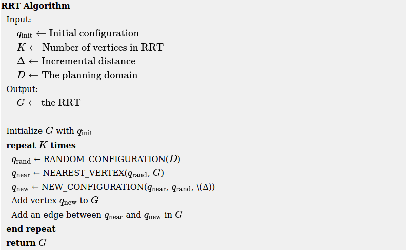
- RANDOM_CONFIGURATION selects a random coordinate in the domain.
- NEAREST_VERTEX finds the vertex in the tree closest to the random coordinate, according to some metric, in this case Euclidian.
- NEW_CONFIGURATION generates a new configuration in the tree by moving distance Δ from the nearest vertex to the randomly selected one.
To view the code, check out the GitHub repo! There is no report as this code was written for the MSR Hackathon. It is included here as RRTs were covered in class.
Particle Filter
The Particle Filter is a nonparametric implementation of a Bayes filter, which computes the posterior $bel(x_t)$ of each state without needing to fit data to a normal distribution. Instead, random state samples (particles) approximate this distibution. This filter is robust to occlusion, nonlinear dynamics, non-Gaussian noise, and most notably, it can represent multimodal posteriors. The basic repeated steps are:
- Generate Initial Particle set $χ_t$ with normally distributed particles. Each particle is a possible robot state.
- Propagate each particle forward with perturbed and noisy controls.
- Perform a weight update if a measurement is recorded.
- Calculate $w_{var}$ , the variance of the set’s weights. $w_{var}$ tending to zero indicates that the weights are converging, discouraging resampling and suggesting creating new particles. A high variance encourages resampling to redistribute weight among particles.
- Extract the posterior from the sample set by computing a weighted average of x, y, and θ using the particle weights. The variance is extracted here for the next iteration.
For more information, please visit the GitHub repo or download the Report
A* (Naive + Online)
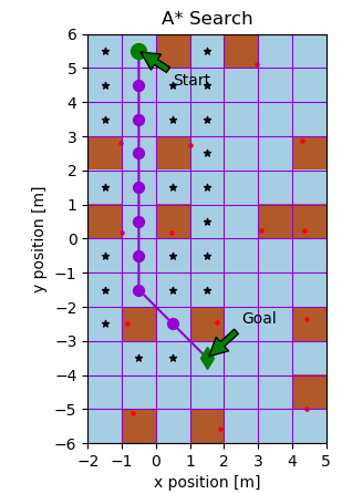
As a form of best-first search, A* evaluates neighbouring nodes using $f(n)=g(n)+h(n)$ where $g(n)$ (usually equal to 1, although $\sqrt{2}$ for diagonal paths showed better performance) is the traversal cost from the current node n to the neighbour node being evaluated, and h(n) is the heuristic cost, which estimates the cheapest path from the current node $n$ to the goal node. Hence, for any given step, the neighbouring node with the lowest f(n) cost will be chosen. If two nodes have the same f (n) cost, they are evaluated by whichever has the lowest h(n) cost [1]. A* search is both complete, meaning that it will always find a solution if one exists, and optimal, meaning that it will always find the cheapest solution in a given set of solutions. For this to be true, the heuristic cost function h(n) must be admissible, meaning that it must never over-estimate the cost to reach the goal. Furthermore, h(n) must be consistent, meaning that the h(n) of parent nodes must always be non-decreasing. Since g(n) represents the true cost to reach a node along a path, an admissible heuristic cost results in f(n) never over-estimating the true cost to the goal [1]. In a grid that allows diagonal movement (i.e each node has a maximum of 8 neighbours), a viable heuristic is the Diagonal Distance Heuristic: $h(n) = D1 ∗ (dx + dy) + (D2 − 2 ∗ D1) ∗ min(dx, dy)$.
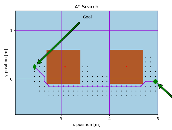
For this project, a naive (basic) A* is implemented for the two figures below, with the expanded nodes shown in black for grid cell sizes of 1 and 0.1 respectively.
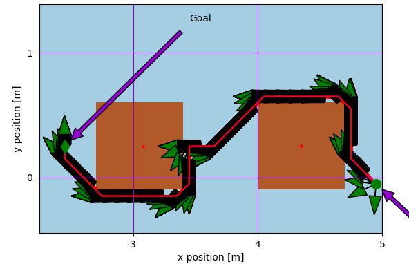
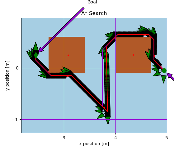
Next, an online A* algorithm was implemented to emulate path planning on a real robot which cannot sense obstacles untill they take up nodes adjacent to it. The figures below show the path traced on a unicycle-modeled robot controlled with a proportional controller, whose heading is portrayed using green arrows. The second figure shows an artificially-induced replan case, whereby the robot’s position was perturbed to show the robustness of the algorithm.
For more information, please visit the GitHub repo or download the Report