1D Maglev Simulation
Summary:
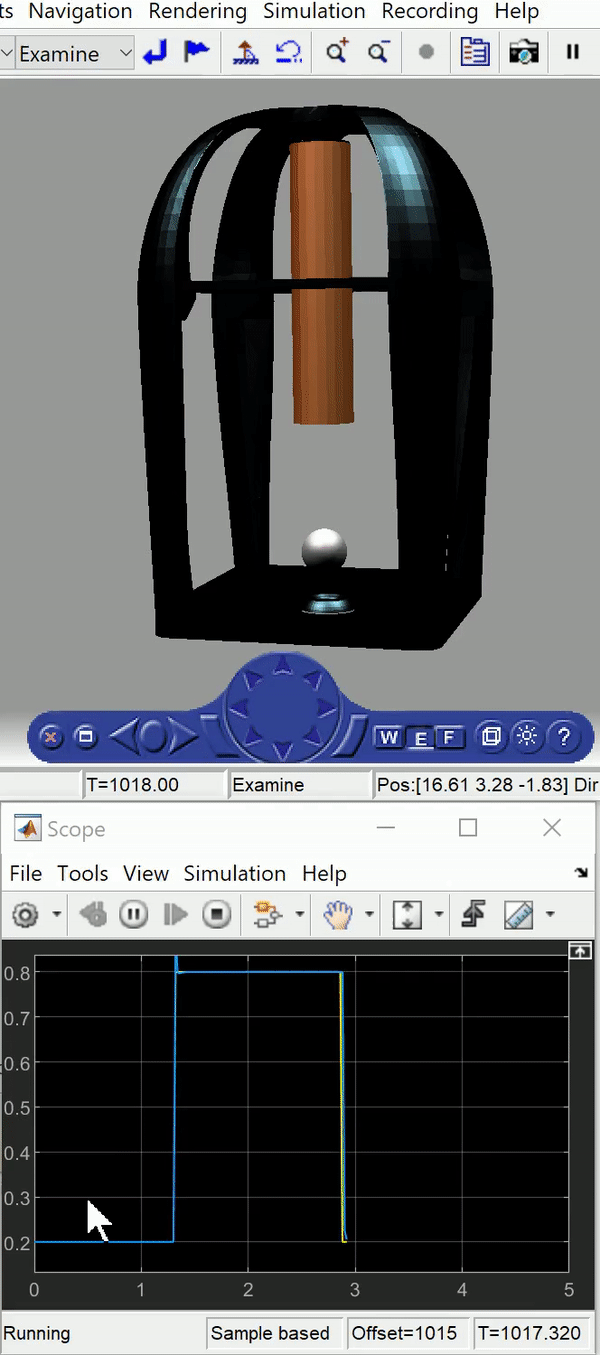
This project focuses on the stable levitation of a steel ball to explore the principles of magnetic levitation and the control theory that underlie the technology. After modeling and developing a test rig was to balance a steel ball in place using one electromagnet, a more complex two dimensional model was then made to actively control the height of the ball as well as its longitudinal travel. For the 1D system a genetic algorithm was used which produced increasingly suitable PID values as it was left to run over time. The algorithm provided a quicker, easier and more accurate solution compared to manual tuning. The 2D model required an cutting-edge control theory; primarily decoupled nonlinear control of inherently coupled systems. The simulation displays the square wave control signal in yellow and the steel ball’s response in blue.
1D System:
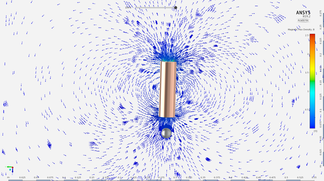
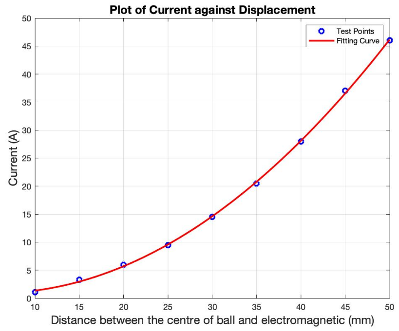
For the 1D System, a state-space model was implemented using first-principles of electromagnetism supplemented by simulations in ANSYS AIM, whereby the ball’s position was altered by a set distance for each trial, and the current required to keep it from falling was recorded using $J=\frac{4I}{D^2}$ where $J$ is flux. This resulted in the equation $I=k(x+x_0)^2$ where $I$ is current, $k$ is a physical system constant, $x_0$ is a system offset, and $x$ is the ball’s displacement from the magnet.
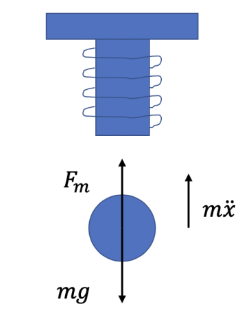
Subsequently, the 1D transfer function was derived via first principles using a free-body-diagram of the system (Figure 4) and a state-space model. The resultant transfer function was \(\frac{U(s)}{X(s)}=G(s)=\frac{767}{s^2-0.7s-1723}\). However, it was found to be unstable as it only had one pole at \(s=41.86\). Spectral factorisation was used to stabilise the function whilst retaining its amplitude information. Using this technique, the denominator of the new transfer function \(f(s)\) was obtained using \(f(s)f(−s)=g(s)g(−s)\) which is an equation on complex plane where g(s) represents the denominator of G(s) , resulting in:
\begin{equation} \frac{U(s)}{X(s)}=F(s)=\frac{64}{s^2+83s+1723} \end{equation}
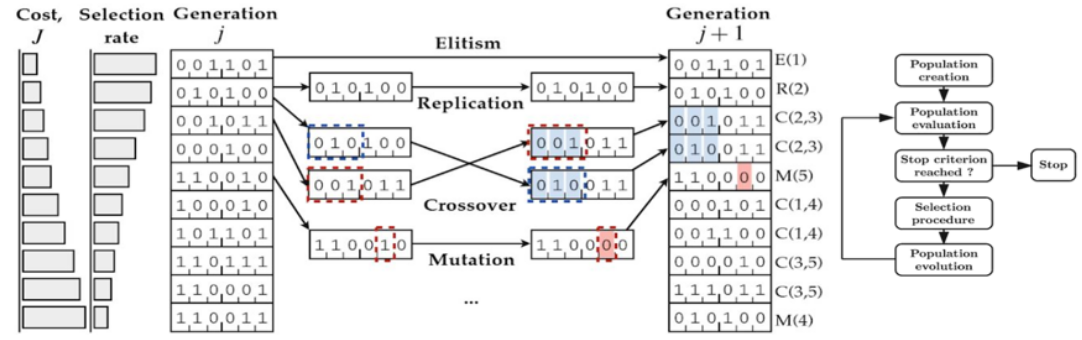
High-Level Map of Genetic Algorithm
1D Controller:
As an alternative to manual tuning, a Genetic Algorithm was used to specify the PID control parameters for the 1D system. As Figure 5 shows, the cost ‘J’ is evaluated for each individual in the population of generation ‘j’ where the selection rate is inversely proportional to the cost produced by each individual. To constitute generation ‘j+1’, four operations can be done:
- Elitism, where the best individual of each generation is immediately passed to the next. This is important because it allows the algorithm to avoid the loss of good solutions due to genetic drift through over-mutation.
- Crossover, where two individuals in the population can exchange some properties and retain others as shown in the figure.
- Replication, whereby a random individual is also passed to the next generation without crossover of properties.
- Mutation can be done whereby a random parameter of the individual is changed to a random value. This allows for a more exhaustive exploration of possible PID values.
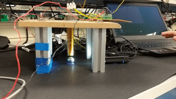
Following from this theory, a simulation was developed in Simulink to test out the controller using a realistic system model shown in the gif at the top of this post. Next, we implemented the setup experimentally as shown in the gif below, which shows an early rig. The second version was prototyped but not completed due to time constraints as the project ran from October to November with no budget.
The report below goes into more detail and explores the modifications made to the control pipeline to improve the rig and adapt it to 2D levitation.