One Small Step For PLEN

Project Overview

For this project, I took the CAD files from the PLEN robot and turned them into OpenAI Gym environments in Pybullet and Gazebo via URDF. Then, I applied Twin-Delayed Deep Deterministic Policy Gradient (TD3) Reinforcement Learning to learn a gait. Finally, I built the real robot and tested my learned policy. If you would like to train your own RL or ZMP algorithm on this robot, please check out the GitHub repository I used OpenAI Gym so you can just plug and play your code!

As the sim-to-real experiment was unsuccessful, I implemented a simple sinewave-based trajectory for the robot’s feet and solved the Inverse Kinematics using this paper. Based on this implementation, I learned that the robot needs wider hips, a lower CoM, and higher-torque motors for any RL policy to be deployed. Here’s a video of the manual trajectory:

The core project components are:

• Pytorch to construct the six deep neural networks required by TD3 Reinforcement Learning.
• PyBullet for simulating the robot and environment.
• RViz and Gazebo for an alternate ROS-based simulation, as well as for constructing and testing the URDF mechanically and dynamically.
• The Real Robot was 3D printed and controlled using a Raspberry Pi Zero W along with 16 servo motors and a 9-axis IMU.

Twin-Delayed Deep Deterministic Policy Gradient:

Most RL focuses on discretised state and action spaces. This poses a problem for robotics, where we generally deal with continuous systems. Building from the continous-applied Deep Deterministic Policy Gradient, TD3 provides a solution to the continuous learning problem.

You should visit OpenAI to learn state-of-the-art RL. I always cross-reference the original papers, but OpenAI’s explanations are more palatable, and they go through the basics too!

Deep Deterministic Policy Gradient

DDPG trains off-policy, and uses the Bellman Equation to learn a Q-function, and uses this to learn a deterministic policy. The algorithm builds on Q-learning, were the optimal action $a^{*}(s)$ is found using $a^{*}(s) = \underset{a}{argmax} Q^{*}(s,a)$, and $Q^{*}(s, a)$ is the optimal action-value function (the * notation denotes optimality).

Computing the max over actions in this function is intractable for continous systems. However, thanks to this continuity of the action space, $Q^{*}(s,a)$ is differentiable with respect to the action argument, suggesting the use of gradient-based learning. Deep Neural Networks (NN) are a convenient way to implement gradient-based learning, and hence, this short introduction derives the name Deep Deterministic Policy Gradient.

$Q^{*}(s,a)$ is described by the bellman equation, where $s’~P$ indicates that the next state $s’$ is sampled through the environment, and $\gamma$ is the discount factor over all future rewards:

Considering a NN $Q_\phi (s,a)$ with parameters $\phi$ alongside a transition set $\Delta$ (s,a,r,s’,d), with r indicating the reward for the state-action pair, and d indicating whether the state $s’$ is terminal, we can use a mean-squared Bellman Error (MSBE) function to tell us how good of an approcimator $Q_\pi$ is for $Q^{*}$. We then minimize this function to approximate $Q^{*}$.

where $r + \gamma (1 - d) \underset{a’}{max} Q_\phi(s’, a’)$ is known as the target, because as we minimize the MSBE loss, we attempt to converge our Q-function towards this target. The problem here is that the target depends on the same parameters $\phi$ that we are trying to train, leading to instability in the minimization. The solution is a target network whose parameters lag $\phi$ using polyak averaging, where the target network is updated as: $\phi_{target} = \rho \phi_{target} + (1 - \rho)\phi$ with $\rho$ between 0 and 1.

With this, our new loss function can be minimized using stochastic gradient descent:

where $\mu_{\theta_{target}}$ is the target policy.

As noted above, the Q-function is differentiable with respect to the continuous action, allowing us to perform gradient ascent with respect to the policy parameters (the Q-function parameters are treated as constants here) to learn a deterministic policy $\mu_{\theta}$, which is another deep NN trained to give us the optimal action for a given state.

Another trick to stabilize learning is to use a replay buffer, which contains a growing set $\Delta$ of previous experiences. Before training even begins, this buffer is populated so that random temporally independent samples can be drawn to avoid training on experiences with sequential correlation, thereby increasing robustness. Finally, since the training is off-policy, normally distributed Gaussian Noise is added to the actions during training. This is to satisfy the exploration-exploitation dillemma, which is especially important for deterministic policies.

Finally, to tie everything together, the below diagram describes the Actor-Critic architecture of the algorithm, where the Q-function is the critic and the policy is the actor. The target networks are not drawn for simplicity.

TD3 Modifications

Two years after the release of the DDPG paper, a modified algorithm was presented with three tricks to combat its main issue: that it consistently over-estimates the Q-Value function by exploiting errors within it.

Clipped Double-Q-Learning

TD3 learns two Q-functions (each with a target network) and uses the smaller of the two to form targets in the MSBE loss function. This brings the total number of NNs in this algorithm from 4 to 6.

Target Policy Smoothing

Noise is also added to the target actions $a’(s’)$, making it harder for the policy to exploit Q-function errors by smoothing out Q along the action space.

Delayed Policy Updates:

One policy update is performed for every two Q-function updates. This is helpful because a better Critic will usually lead to a better Actor, and the former trains the latter.

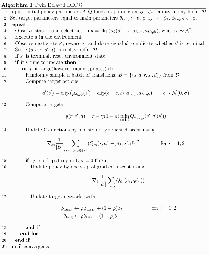
The TD3 algorithm is presented below:

Simulation:

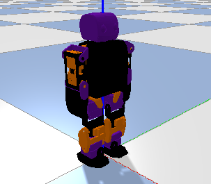
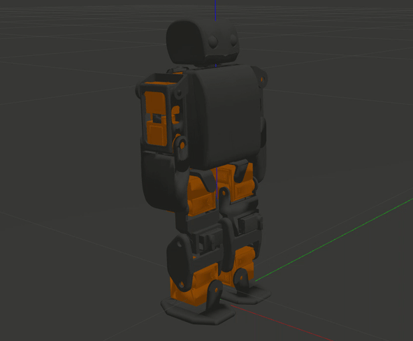
A URDF was built using the STL and inertial properties of CAD plans. First, a Gazebo simulation was built with an OpenAI Gym interface, but it was discovered that Gazebo does not provide controls for stepping into a simulation. The beginnings of a plugin were written, but later scrapped in favor of Pybullet, which is commonly used for RL simulations thanks to its provision of fine temporal control. The Gazebo simulation is still usable for stable systems such as quadrupeds, as the ability to step deterministically is less critical here. The Pybullet and Gazebo environments are shown below.

The system has an 18-dimensional action space for its 18 joints which are mapped from the agent’s [-1, 1] space to the command space. The observation space is 26-dimensional, including the 18 joint positions, the torso’s y,z positions and x velocity, as well as its euler angle rotations and the feet’s simulated contact sensors.

Biologically Inspired Reward Function

Initially, the RL algorithm was heavily exploiting the simulation because multi-contact scenarios are difficult to represent. As a solution, I implemented some elements of human walking into my reward function:

I kept track of the joint-state history and compared the cosine similarity of the hip, knee, and ankle joints between both legs. A value approaching 1 indicates that the joints follow a similar trajectory, and merits a reward. I also penalized the agent if its joint angles did not change between timesteps. In addition, I rewarded the agent for contacting its right foot with the ground during the first half of the gait period, and its left foot during the second half, and added a penalty if both feet were on the ground for more than $33\%$ of the period. Finally, I rewarded the agent for keeping its feet flat as they contacted the ground.

These modifications allowed results to improve for the same number of steps (1,999,999).

Sim To Real:

The real robot was 3D printed and assembled from the CAD files I modified to fit a Raspberry Pi, PWM Board, and IMUwebsite along with 9g servos, as the stock robot fit motors that are unavailable in the US. With the intention of deploying my RL policy, I used servo motors with position feedback, which required an ADC to interface with the Raspberry Pi. Making just the modifications necessary to fit my components resulted in a messy assembly. Additionally, the decision was made not to use the two ‘wrist’ motors as they add almost no functionality and the PWM board I used comes with 16 input pins, and each ADC with 8.

Although the sim-to-real experiment was unsuccessful due to the robot’s dynamic instability, the code is still available for you to run on your own robot. It contains modules to control and read from the servo motors and IMU, as well as an object detection script in OpenCV to estimate the robot’s pose. The main script runs in two modes; it can deploy the RL policy on the robot using the the OpenAI Gym interface, or it can replay a predefined set of joint trajectories. Although the Raspberry Pi is not a real-time system, it was suitable for this application.

Finally, a simple forward trajectory was generated for the robot’s feet relative to its hips, and the complementary joint angles were retrieved using analytical Inverse Kinematics. This includes the standard double and single support phases, and thanks to the symmetry of the walk, it is easy to switch the leading foot.