Project Overview
Three peers and I constructed a syllabus and lecture materials to allow students to construct a motion planning library in C++ from scratch, using ROS’ RViz as a visualization tool. You can view my implementation of the library and the course syllabus on Github. You can also view the lecture presentations here for more detail on each algorithm.
Map Generation
The first part of the library contains two map generation methods, a Probabilistic Roadmap, and a Grid Map.
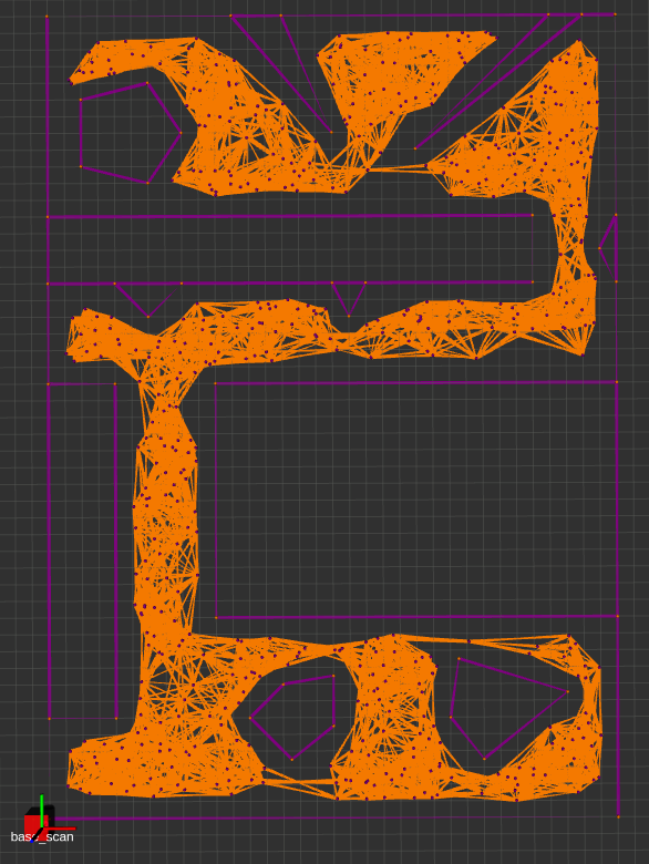
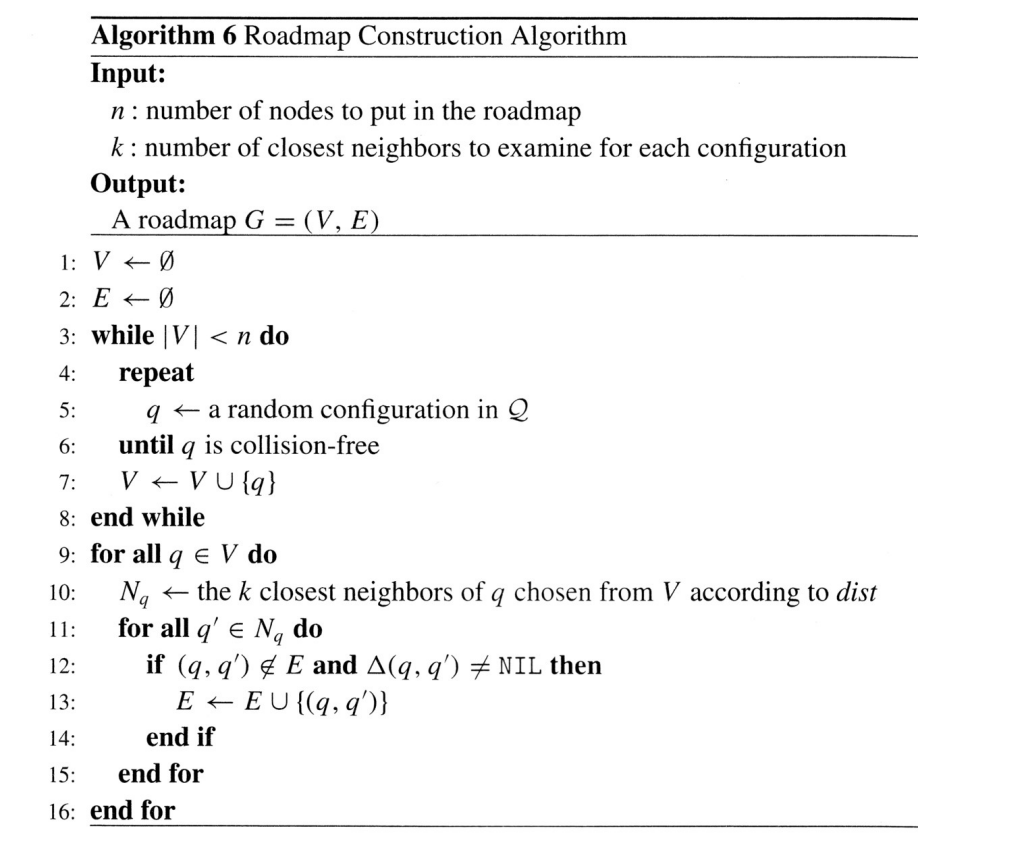
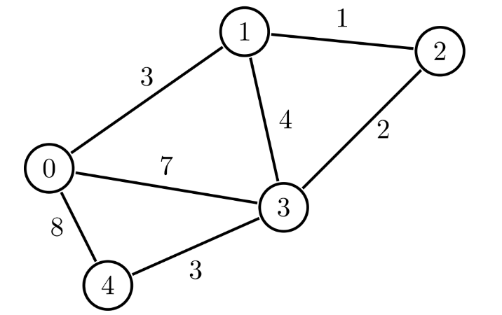
A PRM is an undirected weighted graph characterised by $G = (V, E)$, where Edges $E$, connect pairs of Vertices $V$. Noting that a Vertex can have multiple Edges, below is the algorithm accompanied by a small visual example:
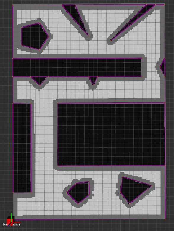
A Grid map is a decomposition of a space into cells (or voxels in higher dimensions), which can be used for row-major-order access. Both of these map types lend themselves well to heuristic search planners, and use the same convex-polygon-based collision detection methods for outlining obstacles and creating a buffer zone suitable for the robot’s size. The PRM lecture covers these methods, and the third Potential Field lecture describes concave-to-convex polygon decomposition.
Global Planners
Heuristic Search
The first set of global planners in this library includes A* , Theta* , LPA* , and D* Lite. The main theme here is that all of these algorithms essentially inherit from A* , which itself optimizes of Djikstra’s Algorithm by introducing a consistent and admissible heuristic to determine the next visited node at each point in the search.
Theta*
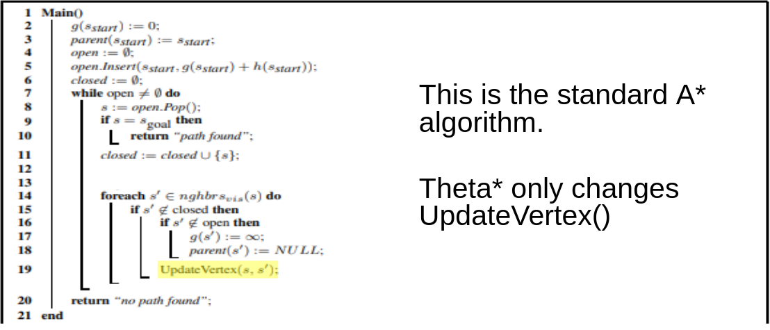
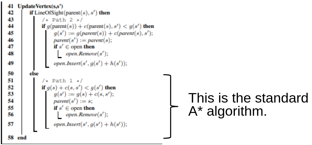
This algorithm - part of the any-angle planner stack - is particularly effective on a PRM. It simply adds the UpdateVertex() method to the A* algorithm for determining whether the current node’s parent can be replace by its grandparent if a line-of-sight exists. The modified algorithm is shown below
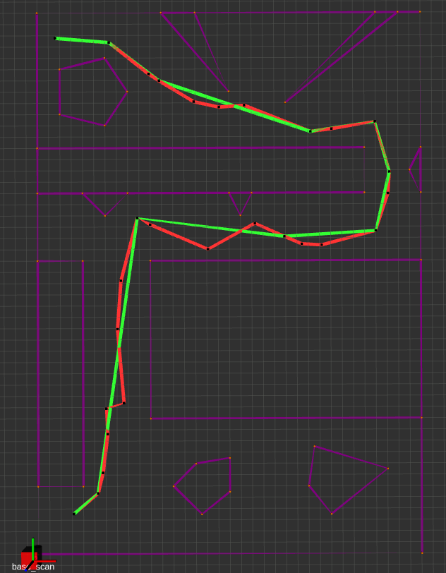
Below, you can see A* (red path) and Theta* (green path) applied to the PRM.
Incremental Planners: LPA* and D* Lite
LPA*
The main idea behind Lifelong Planning A* was to augment A* with the ability to deal with changing maps efficiently. By employing an incremental heuristic search method, as well as additional qualifiers for next-node selection, LPA* is able to plan the exact A* path in a fixed map, and can adapt to map changes without having to re-plan from scratch. It does this by incorporating the concept local consistency using a right-hand-side or rhs(s) cost, where s is a vertex. A locally over-consistent vertex is one whose g(s) cost (the travel cost between successive vertices) is higher than its rhs(s) cost, and vice versa. Hence, the priority queue is only populated with locally inconsistent vertices for evaluation. This alternate approach initially yields the same path as A* would, but the neat trick is that as edge costs change, we can simply update the nodes connected to those modified edges to re-assign parents and construct a new optimal path. Below is an implementation where the map is updated to reveal the true edge costs at some random point on the generated path.
D* Lite
D* Lite is very easy to implement by building off the LPA* scheme. Its namesake, D* (Dynamic A* ) , strives to rework A* for online planning, that is, where the edge costs are unknown until they are revealed by some sensor data on a live robot. To do this - in brief - it is a backwards-search implementation of A* , meaning that it flips the start and goal vertices for planning. There is more to this, and you can consult the lecture notes if you are interested. In D* Lite, however, all we need to do is flip the start and goal vertices in the LPA* algorithm, and everything remains the same. D* Lite also happens to be more efficient than D* . Below is an implementation where the map is updated using a grid-cell visibility radius to emulate sensor readings on the incremented robot pose. Notably, you can see it move towards an infeasible path until it finds out it is blocked, at which point it changes direction.
Local Planners
Potential Fields
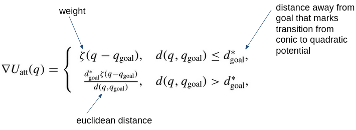
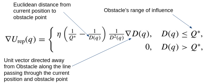
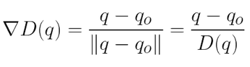
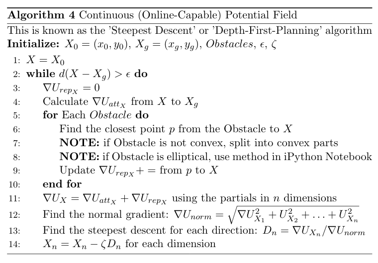
Although technically a global planner, the Potential Fields works well as a local planner. The vanilla implementation is very straigtforward, and is based on gradient descent. In brief, we perform the Steepest Descents algorithm using the Attractive and Repulsive fields shown below. The attractive field is a combination of a conic and quadratic potential, for bounded and continuous differentiability, and the repulsive field is structures for smooth transitions in entering and exiting an obstacle’s field of influence, while providing infinite repulsion at the obstacle boundary. The repulsive field works by finding the closest point between the robot and a given obstacle, which also motivated the description of various concave-to-convex polygon decomposition methods, as this closest point is found using the same method outlined in the PRM lecture.
Here is a gif of the planner in action alongisde the algorithm
Trajectory Optimization
Model Predictive Path Integral Control
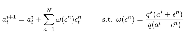
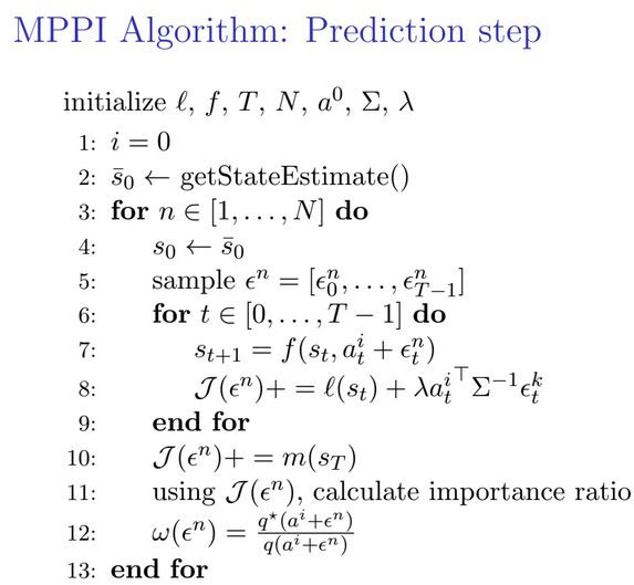
MPPI is a sample-based approach to solving the stochastic Model Predictive Control problem. It works well with highly nonlinear system dynamics as it does not have continuity, differentiability or convexity assumptions. The main idea is to construct an optimal distribution from which we sample an optimal action for the current time step. To do this, we apply Jensen’s Inequality to the Free Energy Formulation, which models how stochastic systems behave in non-equilibrium states. From the fact that a system’s free energy bounds the optimal control problem, we can formulate the optimal control distribution through its probability density function. However, although we cannot directly sample from this distribution, we can use it to evaluate whether action samples are likely optimal by optimizing the system’s KL-Divergence. This gives us a recursive solution based on an importance ratio $\omega$. In terms of tuning, the cost function, action distribution variance and temperature parameter $\lambda$ all impact MPPI’s performance. In particular, $\lambda$ determines the sensitivity of the importance ratio update, where increasing it reduces the resolution of the update in terms of evaluating the costs of adjacent samples. Below is said solution along with the MPPI algorithm:
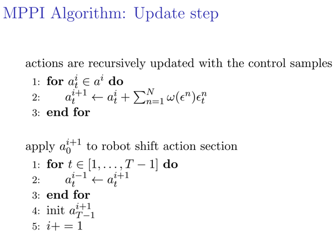
Notably, after the update step, we shift all the actions one timestep down in what is known as a receding horizon. Below is the resultant control for a parallel parking operation on a Differential Drive robot (Turtlebot3) model.
And the associated states and actions (wheel velocities):