Project Overview
This totally-from-scratch project involved modeling a Turtlebot3 in Gazebo and using Differential Drive Kinematics to perform Odometry calculations. The Gazebo Plugin was developed to emulate the low-level interface on the real Turtlebot3 for the ability to develop high-fidelity code in simulation. I also implemented landmark detection on the Turtlebot3’s LIDAR, and used these features to perform EKF SLAM with Unknown Data Association. To use this package, please visit the Github Repository!
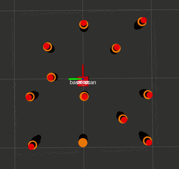
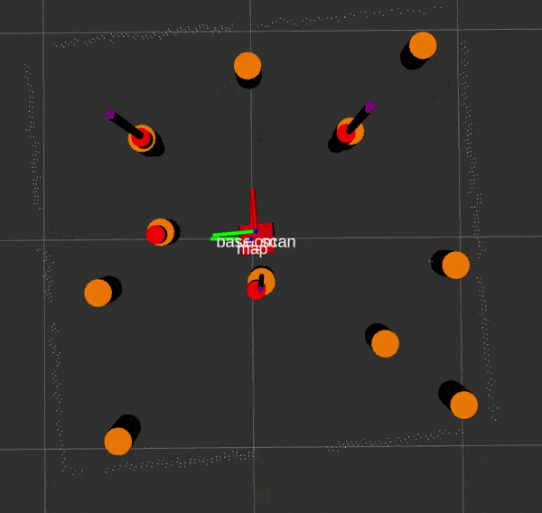
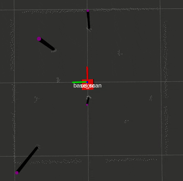
Here is an EKF SLAM run with ground truth and LIDAR landmarks respectively, with Gazebo data in orange, SLAM data in red, and odometry/sensor data in purple.
If you would like to attempt the project on your own, this website by Matthew Elwin contains a host of useful information.
The core project components are:
- rigid2d library containing 2D Lie Group operations for Transforms, Vectors and Twists as well as differential drive robot kinematics for odometry updates.
- nuturtle_description: houses the description of a differential drive robot with a caster wheel for support.
- nuturtle_robot: interfaces with the real Turtlebot3’s low-level controls such as setting wheel speeds and reading sensors.
- nuturtle_gazebo: contains a Gazebo Plugin to emulate the Turtlebot3’s low-level controls in Gazebo for the ability to develop in simulation.
- nuslam: library containing LIDAR feature detection methods and EKF SLAM implementation with Unknown Data Association.
rigid2d:
Chapter 3 of Modern Robotics by Kevin Lynch is a great resource for Transform operations. The implementation in this project is a 2D adaptation of what is presented there, so I will keep my post short by referring to it.
The main operation used in rigid2d’s diff_drive class involves converting to and from Twists and wheel velocities.

twistToWheels();
Beginning with Transforms $T_{1b} = (0, 0, -D)$ and $T_{2b} = (0, 0, D)$ we can extract their Adjoints:
\[A_{1b} = \left[\begin{array}{ccc} 1 & 0 & 0 \\ -D & 1 & 0 \\ 0 & 0 & 1 \end{array} \right]\] \[A_{2b} = \left[\begin{array}{ccc} 1 & 0 & 0 \\ D & 1 & 0 \\ 0 & 0 & 1 \end{array} \right]\]Then, we write Twist $V_b$ in each wheel frame where $V_i = A_{ib} V_b$, noting that $v_y = 0$ for a 2D system:
\[V_1 = \left[\begin{array}{ccc} 1 & 0 & 0 \\ -D & 1 & 0 \\ 0 & 0 & 1 \end{array} \right] \left[\begin{array}{c} w_z \\ v_x \\ v_y \end{array} \right] = \left[\begin{array}{c} w_z \\ -D w_z + v_x \\ v_y \end{array} \right] = \left[\begin{array}{c} w_z \\ r \dot{\phi_1} \\ 0 \end{array} \right]\] \[V_2 = \left[\begin{array}{ccc} 1 & 0 & 0 \\ D & 1 & 0 \\ 0 & 0 & 1 \end{array} \right] \left[\begin{array}{c} w_z \\ v_x \\ v_y \end{array} \right] = \left[\begin{array}{c} w_z \\ D w_z + v_x \\ v_y \end{array} \right] = \left[\begin{array}{c} w_z \\ r \dot{\phi_2} \\ 0 \end{array} \right]\]Hence, we can extract wheel speeds $\dot{\phi_1}$ and $\dot{\phi_2}$:
\[\dot{\phi_1} = \frac{1}{r} \left[\begin{array}{ccc} -D & 1 & 0 \\ \end{array} \right] \left[\begin{array}{c} w_z \\ v_x \\ v_y \end{array} \right]\] \[\dot{\phi_2} = \frac{1}{r} \left[\begin{array}{ccc} D & 1 & 0 \\ \end{array} \right] \left[\begin{array}{c} w_z \\ v_x \\ v_y \end{array} \right]\]wheelsToTwist();
Using the above two equations, we can construct our motion equation matrix:
\[\left[\begin{array}{c} u_L \\ u_R \end{array} \right] = \left[\begin{array}{c} \dot{\phi_1} \\ \dot{\phi_2} \end{array} \right] = \frac{1}{r} \left[\begin{array}{ccc} -D & 1 & 0 \\ D & 1 & 0 \end{array} \right] \left[\begin{array}{c} w_z \\ v_x \\ v_y \end{array} \right]\]where \(H = \frac{1}{r} \left[\begin{array}{ccc} -D & 1 & 0 \\ D & 1 & 0 \end{array} \right]\)
To get our body Twist $V_b$, we compute the pseudo-inverse of H in $V_b = H^+ u$. A column-based attempt ($H^+ = (H^T H)^{-1} H^T$) results in a singular-matrix, so we use a row-based pseudo-invese: $H^+ = H^T (H H^T)^{-1}$ to get
\[H^+ = r \left[\begin{array}{cc} \frac{-1}{2D} & \frac{1}{2D} \\ \frac{1}{2} & \frac{1}{2} \\ 0 & 0 \end{array} \right]\]Finally, our body Twist is:
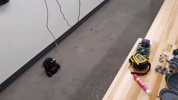
\[V_b = r \left[\begin{array}{cc} \frac{-1}{2D} & \frac{1}{2D} \\ \frac{1}{2} & \frac{1}{2} \\ 0 & 0 \end{array} \right] \left[\begin{array}{c} \dot{\phi_1} \\ \dot{\phi_2} \end{array} \right]\]Here’s an example of the Turtlebot3 moving through waypoints using this library:
nuslam:
LIDAR Feature Detection:
First, a euclidean distance threshold was used to qualify points in the LIDAR point cloud as belonging to the same cluster, with additional logic for wrap-around.
Next, a circle fitting algorithm was used to estimate a centroid and radius for each cluter. Other options are also available.
Additionally, circular classification was attempted to eliminate walls from the set of candidates before performing circle fitting to speed things up, but the algorithm’s performance on noisy point clouds did not merit use.
Here is the landmark detection script in action:
EKF SLAM with Known Data Association:
For EKF SLAM, I refer you to this resource for the details on notation.
Model-based Prediction:
First, we update our state estimate given a Twist using:
\[\hat{\xi_t^{-}} = g(\hat{\xi_{t-1}}, u_t, \epsilon)\]where $\epsilon$ is motion noise, set to zero here, and $^-$ is belief.
Then, we propagate our belief of uncertainty using the state transition model, linearized using Taylor-Series Expansion:
\[\hat{\Sigma_t^-} = g'(\hat{\xi_{t-1}}, u_t, \epsilon) \hat{\Sigma_{t-1}} g'(\hat{\xi_{t-1}}, u_t, \epsilon)^T + \bar{Q}\]where our process noise, \(\bar{Q} = \left[\begin{array}{cc} Q & 0_{3\times 2n} \\ 0_{2n\times 3} & 0_{2n \times 2n} \end{array} \right]\)
and $Q$ is a diagonal matrix of sampled Gaussian noise for $x,y,\theta$.
Measurement Update:
For landmark $j$ associated for measurement $i$:
First, compute the Kalman Gain $K_i$ from the linearized measurement model:
\[K_i = \Sigma_t^- h_j'(\xi_t)^T (h_j'(\xi_t) \Sigma_t^- h_j'(\xi_t)^T + R)^{-1}\]where R is a diagonal measurement noise matrix.
Then, after computing the theoretical measurement using $\hat{z_t^i} = h_j(\hat{\xi_t^-})$, get the posterior state update:
\[\hat{\xi_t} = \hat{\xi_t^-} + K_i (z_t^i - \hat{z_t^i})\]and the posterior covariance:
\[\Sigma_t = (I - K_i h_j'(\xi_t)) \Sigma_t^-\]Note that this algorithm is written such that we perform our full EKF SLAM update once we have received both odometry and measurement data. Take a look at slam.cpp in the nuslam package to see how this is done.
Data Association using Mahalanobis Distance:
For Data Association, I refer you to this resource for details on notation.
This algorithm is placed just before the measurement update step:
for $k = 0$ to $k < N$: (where N is the number of landmarks seen so far)
compute $\psi_k = h_k’(\hat{\xi_t^-}) \Sigma_t^- h_k’(\hat{\xi_t^-})^T + R $
calculate the predicted measurement $\hat{z_t^k}$, and finally, compute the mahalanobis distance $d_k = (z_i - \hat{z_k}) \psi_k (z_i - \hat{z_k})^T$
append to vector of measurements
endfor
Next, before computing the measurement update, find $d^*$, the smallest mahalanobis distance in the vector, and $j$, its index.
If $d^{*}$ is smaller than the lower-bound mahalanobis threshold, then j is the index used in the measurement update. If it is greater the the upper-bound mahalanobis threshold, then $j = N$ and $N$ is subsequently incremented.